Clinical Reporting with {gtsummary}
Introduction
Daniel D. Sjoberg

How it started
Began to address reproducible issues while working in academia
Goal was to build a package to summarize study results with code that was both simple and customizable
First release in May 2019
How it’s going
The stats
- 1,300,000+ installations from CRAN
- 1100+ GitHub stars
- 300+ contributors
- 50+ code contributors
Won the 2021 American Statistical Association (ASA) Innovation in Programming Award
Won the 2024 Posit Pharma Table Contest
![]()


{gtsummary} overview
- Create tabular summaries with sensible defaults but highly customizable
- Types of summaries:
- “Table 1”-types
- Cross-tabulation
- Regression models
- Survival data
- Survey data
- Custom tables
- Report statistics from {gtsummary} tables inline in R Markdown
- Stack and/or merge any table type
- Use themes to standardize across tables
- Choose from different print engines
Example Dataset
The
trialdata set is included with {gtsummary}Simulated data set of baseline characteristics for 200 patients who receive Drug A or Drug B
Variables were assigned labels using the
labelledpackage
| Chemotherapy Treatment | Age | Marker Level (ng/mL) | T Stage | Grade | Tumor Response | Patient Died | Months to Death/Censor |
|---|---|---|---|---|---|---|---|
| Drug A | 23 | 0.160 | T1 | II | 0 | 0 | 24.00 |
| Drug B | 9 | 1.107 | T2 | I | 1 | 0 | 24.00 |
| Drug A | 31 | 0.277 | T1 | II | 0 | 0 | 24.00 |
| Drug A | NA | 2.067 | T3 | III | 1 | 1 | 17.64 |
| Drug A | 51 | 2.767 | T4 | III | 1 | 1 | 16.43 |
| Drug B | 39 | 0.613 | T4 | I | 0 | 1 | 15.64 |
Example Dataset
tbl_summary()
Basic tbl_summary()
| Characteristic | N = 2001 |
|---|---|
| Age | 47 (38, 57) |
| Unknown | 11 |
| Grade | |
| I | 68 (34%) |
| II | 68 (34%) |
| III | 64 (32%) |
| Tumor Response | 61 (32%) |
| Unknown | 7 |
| 1 Median (Q1, Q3); n (%) | |
Four types of summaries:
continuous,continuous2,categorical, anddichotomousStatistics are
median (IQR)for continuous,n (%)for categorical/dichotomousVariables coded
0/1,TRUE/FALSE,Yes/Notreated as dichotomousLists
NAvalues under “Unknown”Label attributes are printed automatically
Customize tbl_summary() output
| Characteristic | Drug A N = 981 |
Drug B N = 1021 |
|---|---|---|
| Age | 46 (37, 60) | 48 (39, 56) |
| Unknown | 7 | 4 |
| Grade | ||
| I | 35 (36%) | 33 (32%) |
| II | 32 (33%) | 36 (35%) |
| III | 31 (32%) | 33 (32%) |
| Tumor Response | 28 (29%) | 33 (34%) |
| Unknown | 3 | 4 |
| 1 Median (Q1, Q3); n (%) | ||
by: specify a column variable for cross-tabulation
Customize tbl_summary() output
| Characteristic | Drug A N = 981 |
Drug B N = 1021 |
|---|---|---|
| Age | ||
| Median (Q1, Q3) | 46 (37, 60) | 48 (39, 56) |
| Unknown | 7 | 4 |
| Grade | ||
| I | 35 (36%) | 33 (32%) |
| II | 32 (33%) | 36 (35%) |
| III | 31 (32%) | 33 (32%) |
| Tumor Response | 28 (29%) | 33 (34%) |
| Unknown | 3 | 4 |
| 1 n (%) | ||
by: specify a column variable for cross-tabulationtype: specify the summary type
Customize tbl_summary() output
| Characteristic | Drug A N = 981 |
Drug B N = 1021 |
|---|---|---|
| Age | ||
| Mean (SD) | 47 (15) | 47 (14) |
| Min, Max | 6, 78 | 9, 83 |
| Unknown | 7 | 4 |
| Grade | ||
| I | 35 (36%) | 33 (32%) |
| II | 32 (33%) | 36 (35%) |
| III | 31 (32%) | 33 (32%) |
| Tumor Response | 28 / 95 (29%) | 33 / 98 (34%) |
| Unknown | 3 | 4 |
| 1 n (%); n / N (%) | ||
by: specify a column variable for cross-tabulationtype: specify the summary typestatistic: customize the reported statistics
Customize tbl_summary() output
| Characteristic | Drug A N = 981 |
Drug B N = 1021 |
|---|---|---|
| Age | ||
| Mean (SD) | 47 (15) | 47 (14) |
| Min, Max | 6, 78 | 9, 83 |
| Unknown | 7 | 4 |
| Pathologic tumor grade | ||
| I | 35 (36%) | 33 (32%) |
| II | 32 (33%) | 36 (35%) |
| III | 31 (32%) | 33 (32%) |
| Tumor Response | 28 / 95 (29%) | 33 / 98 (34%) |
| Unknown | 3 | 4 |
| 1 n (%); n / N (%) | ||
by: specify a column variable for cross-tabulationtype: specify the summary typestatistic: customize the reported statistics
label: change or customize variable labels
Customize tbl_summary() output
| Characteristic | Drug A N = 981 |
Drug B N = 1021 |
|---|---|---|
| Age | ||
| Mean (SD) | 47.0 (14.7) | 47.4 (14.0) |
| Min, Max | 6.0, 78.0 | 9.0, 83.0 |
| Unknown | 7 | 4 |
| Pathologic tumor grade | ||
| I | 35 (36%) | 33 (32%) |
| II | 32 (33%) | 36 (35%) |
| III | 31 (32%) | 33 (32%) |
| Tumor Response | 28 / 95 (29%) | 33 / 98 (34%) |
| Unknown | 3 | 4 |
| 1 n (%); n / N (%) | ||
by: specify a column variable for cross-tabulationtype: specify the summary typestatistic: customize the reported statistics
label: change or customize variable labelsdigits: specify the number of decimal places for rounding
{gtsummary} + formulas
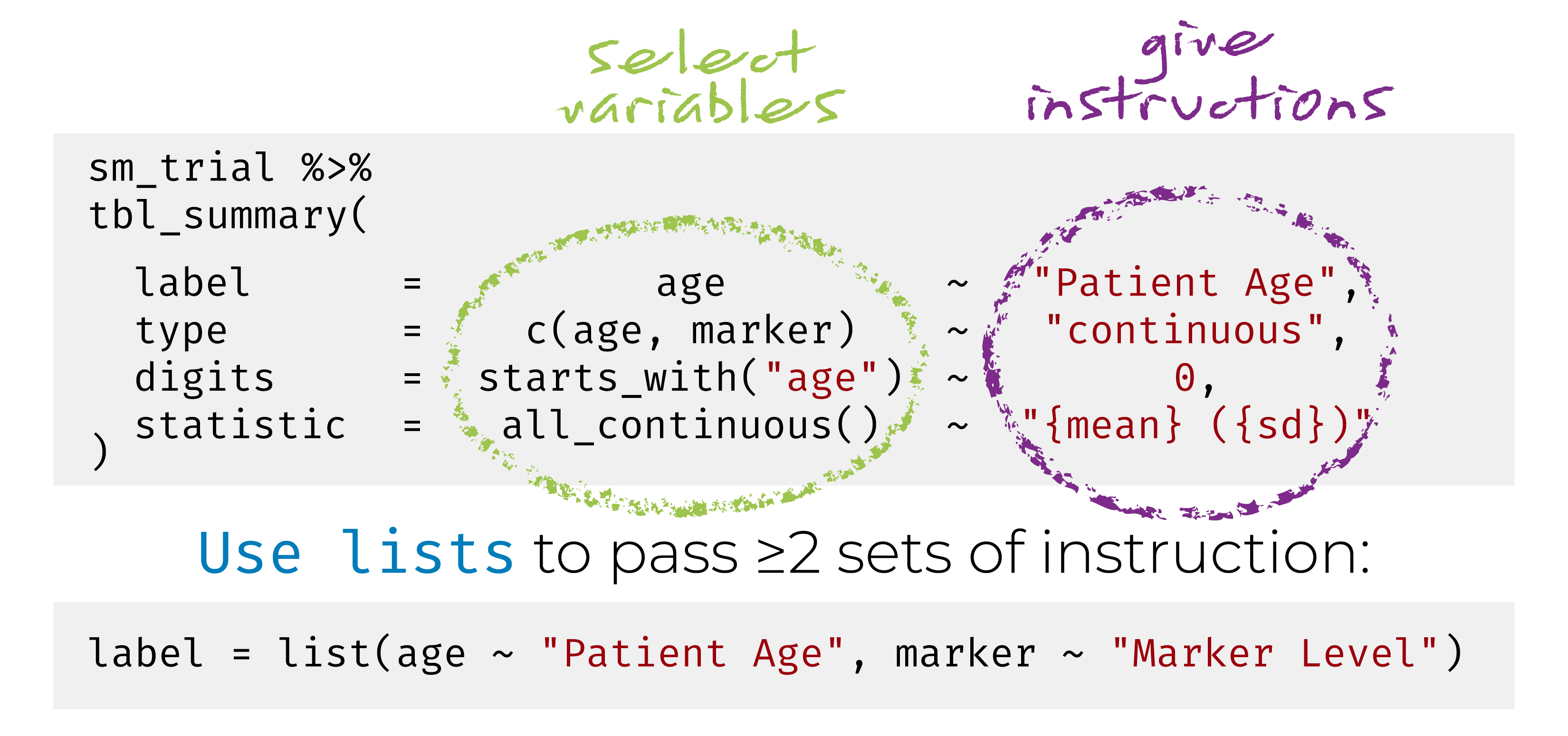
Named list are OK too! label = list(age = "Patient Age")
Add-on functions in {gtsummary}
tbl_summary() objects can also be updated using related functions.
add_*()add additional column of statistics or information, e.g. p-values, q-values, overall statistics, treatment differences, N obs., and moremodify_*()modify table headers, spanning headers, footnotes, and morebold_*()/italicize_*()style labels, variable levels, significant p-values
Update tbl_summary() with add_*()
| Characteristic | Drug A N = 981 |
Drug B N = 1021 |
p-value2 | q-value3 |
|---|---|---|---|---|
| Age | 46 (37, 60) | 48 (39, 56) | 0.7 | 0.9 |
| Unknown | 7 | 4 | ||
| Grade | 0.9 | 0.9 | ||
| I | 35 (36%) | 33 (32%) | ||
| II | 32 (33%) | 36 (35%) | ||
| III | 31 (32%) | 33 (32%) | ||
| Tumor Response | 28 (29%) | 33 (34%) | 0.5 | 0.9 |
| Unknown | 3 | 4 | ||
| 1 Median (Q1, Q3); n (%) | ||||
| 2 Wilcoxon rank sum test; Pearson’s Chi-squared test | ||||
| 3 False discovery rate correction for multiple testing | ||||
add_p(): adds a column of p-valuesadd_q(): adds a column of p-values adjusted for multiple comparisons through a call top.adjust()
Update tbl_summary() with add_*()
| Characteristic | Overall N = 2001 |
Drug A N = 981 |
Drug B N = 1021 |
|---|---|---|---|
| Age | 47 (38, 57) | 46 (37, 60) | 48 (39, 56) |
| Grade | |||
| I | 68 (34%) | 35 (36%) | 33 (32%) |
| II | 68 (34%) | 32 (33%) | 36 (35%) |
| III | 64 (32%) | 31 (32%) | 33 (32%) |
| Tumor Response | 61 (32%) | 28 (29%) | 33 (34%) |
| 1 Median (Q1, Q3); n (%) | |||
add_overall(): adds a column of overall statistics
Update tbl_summary() with add_*()
| Characteristic | N | Overall N = 2001 |
Drug A N = 981 |
Drug B N = 1021 |
|---|---|---|---|---|
| Age | 189 | 47 (38, 57) | 46 (37, 60) | 48 (39, 56) |
| Grade | 200 | |||
| I | 68 (34%) | 35 (36%) | 33 (32%) | |
| II | 68 (34%) | 32 (33%) | 36 (35%) | |
| III | 64 (32%) | 31 (32%) | 33 (32%) | |
| Tumor Response | 193 | 61 (32%) | 28 (29%) | 33 (34%) |
| 1 Median (Q1, Q3); n (%) | ||||
add_overall(): adds a column of overall statisticsadd_n(): adds a column with the sample size
Update tbl_summary() with add_*()
| Characteristic | N | Overall N = 200 |
Drug A N = 98 |
Drug B N = 102 |
|---|---|---|---|---|
| Age, Median (Q1, Q3) | 189 | 47 (38, 57) | 46 (37, 60) | 48 (39, 56) |
| Grade, No. (%) | 200 | |||
| I | 68 (34%) | 35 (36%) | 33 (32%) | |
| II | 68 (34%) | 32 (33%) | 36 (35%) | |
| III | 64 (32%) | 31 (32%) | 33 (32%) | |
| Tumor Response, No. (%) | 193 | 61 (32%) | 28 (29%) | 33 (34%) |
add_overall(): adds a column of overall statisticsadd_n(): adds a column with the sample sizeadd_stat_label(): adds a description of the reported statistic
Update with bold_*()/italicize_*()
| Characteristic | Drug A N = 981 |
Drug B N = 1021 |
p-value2 |
|---|---|---|---|
| Age | 46 (37, 60) | 48 (39, 56) | 0.7 |
| Unknown | 7 | 4 | |
| Grade | 0.9 | ||
| I | 35 (36%) | 33 (32%) | |
| II | 32 (33%) | 36 (35%) | |
| III | 31 (32%) | 33 (32%) | |
| Tumor Response | 28 (29%) | 33 (34%) | 0.5 |
| Unknown | 3 | 4 | |
| 1 Median (Q1, Q3); n (%) | |||
| 2 Wilcoxon rank sum test; Pearson’s Chi-squared test | |||
bold_labels(): bold the variable labelsitalicize_levels(): italicize the variable levelsbold_p(): bold p-values according a specified threshold
Update tbl_summary() with modify_*()
| Characteristic |
Drug
|
|
|---|---|---|
| Group A1 | Group B1 | |
| Age | 46 (37, 60) | 48 (39, 56) |
| Grade | ||
| I | 35 (36%) | 33 (32%) |
| II | 32 (33%) | 36 (35%) |
| III | 31 (32%) | 33 (32%) |
| Tumor Response | 28 (29%) | 33 (34%) |
| 1 median (IQR) for continuous; n (%) for categorical | ||
- Use
show_header_names()to see the internal header names available for use inmodify_header()
Column names
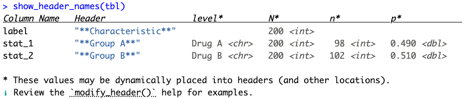
all_stat_cols() selects columns "stat_1" and "stat_2"
For example, the code below would set the first header to “Drug A, N = 98” and the second to “Drug B, N = 102”.
Update tbl_summary() with add_*()
trial |>
  select(trt, marker, response) |>
  tbl_summary(
    by = trt,
    statistic = list(marker ~ "{mean} ({sd})",
                     response ~ "{p}%"),
    missing = "no"
  ) |>
add_difference()| Characteristic | Drug A N = 981 |
Drug B N = 1021 |
Difference2 | 95% CI2 | p-value2 |
|---|---|---|---|---|---|
| Marker Level (ng/mL) | 1.02 (0.89) | 0.82 (0.83) | 0.20 | -0.05, 0.44 | 0.12 |
| Tumor Response | 29% | 34% | -4.2% | -18%, 9.9% | 0.6 |
| Abbreviation: CI = Confidence Interval | |||||
| 1 Mean (SD); % | |||||
| 2 Welch Two Sample t-test; 2-sample test for equality of proportions with continuity correction | |||||
add_difference(): mean and rate differences between two groups. Can also be adjusted differences
Update tbl_summary() with add_*()
Add-on functions in {gtsummary}
And many more!
See the documentation at http://www.danieldsjoberg.com/gtsummary/reference/index.html
And a detailed tbl_summary() vignette at http://www.danieldsjoberg.com/gtsummary/articles/tbl_summary.html
Cross-tabulation with tbl_cross()
tbl_cross() is a wrapper for tbl_summary() for n x m tables
Continuous Summaries with tbl_continuous()
tbl_continuous() summarizes a continuous variable by 1, 2, or more categorical variables
Survey data with tbl_svysummary()
| Characteristic |
Survived
|
p-value2 | |
|---|---|---|---|
| No N = 1,4901 |
Yes N = 7111 |
||
| Class | 0.7 | ||
| 1st | 122 (8.2%) | 203 (29%) | |
| 2nd | 167 (11%) | 118 (17%) | |
| 3rd | 528 (35%) | 178 (25%) | |
| Crew | 673 (45%) | 212 (30%) | |
| Sex | 0.048 | ||
| Male | 1,364 (92%) | 367 (52%) | |
| Female | 126 (8.5%) | 344 (48%) | |
| 1 n (%) | |||
| 2 Pearson’s X^2: Rao & Scott adjustment | |||
Survival outcomes with tbl_survfit()
library(survival)
fit <- survfit(Surv(ttdeath, death) ~ trt, trial)

tbl_survfit(
  fit,
  times = c(12, 24),
  label_header = "**{time} Month**"
) |>
add_p()| Characteristic | 12 Month | 24 Month | p-value1 |
|---|---|---|---|
| Chemotherapy Treatment | 0.2 | ||
| Drug A | 91% (85%, 97%) | 47% (38%, 58%) | |
| Drug B | 86% (80%, 93%) | 41% (33%, 52%) | |
| 1 Log-rank test | |||
Nested summaries with tbl_hierarchical()
ADAE_subset <- cards::ADAE |> dplyr::filter(AESOC %in% unique(cards::ADAE$AESOC)[1:5], AETERM %in% unique(cards::ADAE$AETERM)[1:5], startsWith(TRTA, "X"))

tbl_hierarchical(
  data = ADAE_subset,
  variables = c(AESOC, AETERM),
  by = TRTA,
  denominator = cards::ADSL |> mutate(TRTA = ARM),
  id = USUBJID
)| Primary System Organ Class Reported Term for the Adverse Event |
Xanomeline High Dose N = 841 |
Xanomeline Low Dose N = 841 |
|---|---|---|
| CARDIAC DISORDERS | 3 (3.6%) | 0 (0%) |
| ATRIOVENTRICULAR BLOCK SECOND DEGREE | 3 (3.6%) | 0 (0%) |
| GASTROINTESTINAL DISORDERS | 4 (4.8%) | 5 (6.0%) |
| DIARRHOEA | 4 (4.8%) | 5 (6.0%) |
| GENERAL DISORDERS AND ADMINISTRATION SITE CONDITIONS | 25 (30%) | 24 (29%) |
| APPLICATION SITE ERYTHEMA | 15 (18%) | 12 (14%) |
| APPLICATION SITE PRURITUS | 22 (26%) | 22 (26%) |
| SKIN AND SUBCUTANEOUS TISSUE DISORDERS | 14 (17%) | 15 (18%) |
| ERYTHEMA | 14 (17%) | 15 (18%) |
| 1 n (%) | ||
tbl_regression()
Traditional model summary()
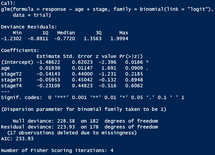
Looks messy and it’s not easy to digest
Basic tbl_regression()
| Characteristic | log(OR) | 95% CI | p-value |
|---|---|---|---|
| Age | 0.02 | 0.00, 0.04 | 0.091 |
| T Stage | |||
| T1 | — | — | |
| T2 | -0.54 | -1.4, 0.31 | 0.2 |
| T3 | -0.06 | -0.95, 0.82 | 0.9 |
| T4 | -0.23 | -1.1, 0.64 | 0.6 |
| Abbreviations: CI = Confidence Interval, OR = Odds Ratio | |||
Displays p-values for covariates
Shows reference levels for categorical variables
Model type recognized as logistic regression with odds ratio appearing in header
Customize tbl_regression() output
| Characteristic | OR | 95% CI | p-value |
|---|---|---|---|
| Age | 1.02 | 1.00, 1.04 | 0.087 |
| T Stage | 0.6 | ||
| T1 | — | — | |
| T2 | 0.58 | 0.24, 1.37 | |
| T3 | 0.94 | 0.39, 2.28 | |
| T4 | 0.79 | 0.33, 1.90 | |
| No. Obs. | 183 | ||
| Log-likelihood | -112 | ||
| AIC | 234 | ||
| BIC | 250 | ||
| Abbreviations: CI = Confidence Interval, OR = Odds Ratio | |||
Display odds ratio estimates and confidence intervals
Add global p-values
Add various model statistics
Supported models in tbl_regression()
betareg::betareg(), biglm::bigglm(), brms::brm(), cmprsk::crr(), fixest::feglm(), fixest::femlm(), fixest::feNmlm(), fixest::feols(), gam::gam(), geepack::geeglm(), glmmTMB::glmmTMB(), glmtoolbox::glmgee(), lavaan::lavaan(), lfe::felm(), lme4::glmer.nb(), lme4::glmer(), lme4::lmer(), logitr::logitr(), MASS::glm.nb(), MASS::polr(), mgcv::gam(), mice::mira, mmrm::mmrm(), multgee::nomLORgee(), multgee::ordLORgee(), nnet::multinom(), ordinal::clm(), ordinal::clmm(), parsnip::model_fit, plm::plm(), pscl::hurdle(), pscl::zeroinfl(), rstanarm::stan_glm(), stats::aov(), stats::glm(), stats::lm(), stats::nls(), survey::svycoxph(), survey::svyglm(), survey::svyolr(), survival::cch(), survival::clogit(), survival::coxph(), survival::survreg(), tidycmprsk::crr(), VGAM::vgam(), VGAM::vglm()
Custom tidiers can be written and passed to tbl_regression() using the tidy_fun= argument.
Univariate models with tbl_uvregression()
| Characteristic | N | OR | 95% CI | p-value |
|---|---|---|---|---|
| Chemotherapy Treatment | 193 | |||
| Drug A | — | — | ||
| Drug B | 1.21 | 0.66, 2.24 | 0.5 | |
| Age | 183 | 1.02 | 1.00, 1.04 | 0.10 |
| Grade | 193 | |||
| I | — | — | ||
| II | 0.95 | 0.45, 2.00 | 0.9 | |
| III | 1.10 | 0.52, 2.29 | 0.8 | |
| Abbreviations: CI = Confidence Interval, OR = Odds Ratio | ||||
Specify model
method,method.args, and theresponsevariableArguments and helper functions like
exponentiate,bold_*(),add_global_p()can also be used withtbl_uvregression()
Break

inline_text()
{gtsummary} reporting with inline_text()
Tables are important, but we often need to report results in-line.
Any statistic reported in a {gtsummary} table can be extracted and reported in-line in an R Markdown document with the
inline_text()function.The pattern of what is reported can be modified with the
pattern=argument.Default is
pattern = "{estimate} ({conf.level*100}% CI {conf.low}, {conf.high}; {p.value})"for regression summaries.
{gtsummary} reporting with inline_text()
| Characteristic | N | OR | 95% CI | p-value |
|---|---|---|---|---|
| Chemotherapy Treatment | 193 | |||
| Drug A | — | — | ||
| Drug B | 1.21 | 0.66, 2.24 | 0.5 | |
| Age | 183 | 1.02 | 1.00, 1.04 | 0.10 |
| Grade | 193 | |||
| I | — | — | ||
| II | 0.95 | 0.45, 2.00 | 0.9 | |
| III | 1.10 | 0.52, 2.29 | 0.8 | |
| Abbreviations: CI = Confidence Interval, OR = Odds Ratio | ||||
In Code: The odds ratio for age is `r inline_text(tbl_uvreg, variable = age)`
In Report: The odds ratio for age is 1.02 (95% CI 1.00, 1.04; p=0.10)
tbl_merge()/tbl_stack()
tbl_merge() for side-by-side tables
A univariable table:
tbl_uvsurv <-
  trial |>
  select(age, grade, death, ttdeath) |>
  tbl_uvregression(
    method = coxph,
    y = Surv(ttdeath, death),
    exponentiate = TRUE
  ) |>
  add_global_p()
tbl_uvsurv| Characteristic | N | HR | 95% CI | p-value |
|---|---|---|---|---|
| Age | 189 | 1.01 | 0.99, 1.02 | 0.3 |
| Grade | 200 | 0.075 | ||
| I | — | — | ||
| II | 1.28 | 0.80, 2.05 | ||
| III | 1.69 | 1.07, 2.66 | ||
| Abbreviations: CI = Confidence Interval, HR = Hazard Ratio | ||||
A multivariable table:
tbl_mvsurv <-
  coxph(
    Surv(ttdeath, death) ~ age + grade,
    data = trial
  ) |>
  tbl_regression(
    exponentiate = TRUE
  ) |>
  add_global_p()
tbl_mvsurv| Characteristic | HR | 95% CI | p-value |
|---|---|---|---|
| Age | 1.01 | 0.99, 1.02 | 0.3 |
| Grade | 0.041 | ||
| I | — | — | |
| II | 1.20 | 0.73, 1.97 | |
| III | 1.80 | 1.13, 2.87 | |
| Abbreviations: CI = Confidence Interval, HR = Hazard Ratio | |||
tbl_merge() for side-by-side tables
| Characteristic |
Univariable
|
Multivariable
|
|||||
|---|---|---|---|---|---|---|---|
| N | HR | 95% CI | p-value | HR | 95% CI | p-value | |
| Age | 189 | 1.01 | 0.99, 1.02 | 0.3 | 1.01 | 0.99, 1.02 | 0.3 |
| Grade | 200 | 0.075 | 0.041 | ||||
| I | — | — | — | — | |||
| II | 1.28 | 0.80, 2.05 | 1.20 | 0.73, 1.97 | |||
| III | 1.69 | 1.07, 2.66 | 1.80 | 1.13, 2.87 | |||
| Abbreviations: CI = Confidence Interval, HR = Hazard Ratio | |||||||
tbl_stack() to combine vertically
A univariable table:
tbl_uvsurv2 <-
  coxph(Surv(ttdeath, death) ~ trt,
        data = trial) |>
  tbl_regression(
    show_single_row = trt,
    label = trt ~ "Drug B vs A",
    exponentiate = TRUE
  )
tbl_uvsurv2| Characteristic | HR | 95% CI | p-value |
|---|---|---|---|
| Drug B vs A | 1.25 | 0.86, 1.81 | 0.2 |
| Abbreviations: CI = Confidence Interval, HR = Hazard Ratio | |||
A multivariable table:
tbl_mvsurv2 <-
  coxph(Surv(ttdeath, death) ~
          trt + grade + stage + marker,
        data = trial) |>
  tbl_regression(
    show_single_row = trt,
    label = trt ~ "Drug B vs A",
    exponentiate = TRUE,
    include = "trt"
  )
tbl_mvsurv2| Characteristic | HR | 95% CI | p-value |
|---|---|---|---|
| Drug B vs A | 1.30 | 0.88, 1.92 | 0.2 |
| Abbreviations: CI = Confidence Interval, HR = Hazard Ratio | |||
tbl_stack() to combine vertically
tbl_strata() for stratified tables
sm_trial |>
  mutate(grade = paste("Grade", grade)) |>
  tbl_strata(
    strata = grade,
    ~tbl_summary(.x, by = trt, missing = "no") |>
      modify_header(all_stat_cols() ~ "**{level}**")
)| Characteristic |
Grade I
|
Grade II
|
Grade III
|
|||
|---|---|---|---|---|---|---|
| Drug A1 | Drug B1 | Drug A1 | Drug B1 | Drug A1 | Drug B1 | |
| Age | 46 (36, 60) | 48 (42, 55) | 45 (31, 55) | 51 (42, 58) | 52 (42, 61) | 45 (36, 52) |
| Tumor Response | 8 (23%) | 13 (41%) | 7 (23%) | 12 (36%) | 13 (43%) | 8 (24%) |
| 1 Median (Q1, Q3); n (%) | ||||||
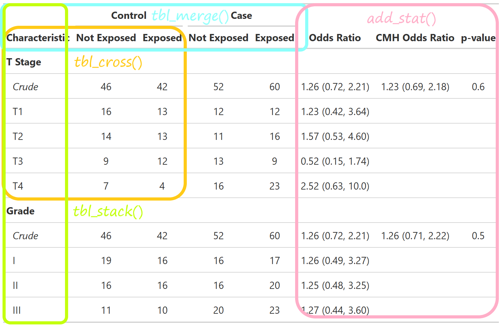
Define custom function tbl_cmh()
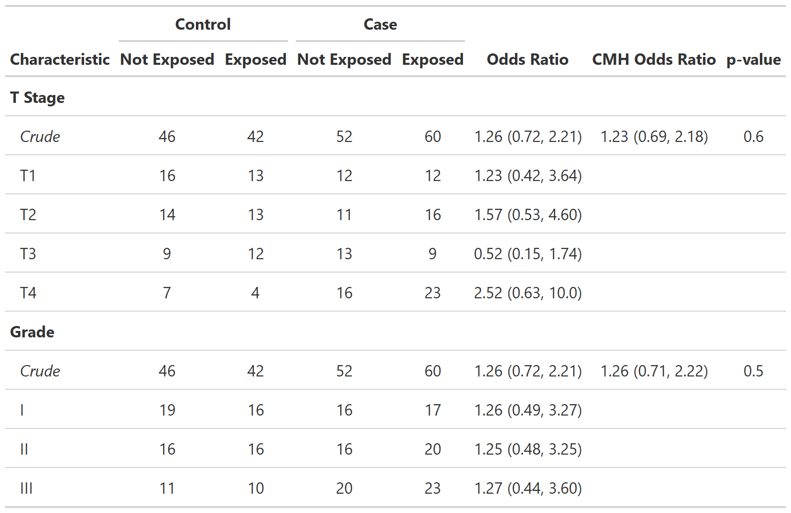
Define custom function tbl_cmh()
{gtsummary} themes
{gtsummary} theme basics
A theme is a set of customization preferences that can be easily set and reused.
Themes control default settings for existing functions
Themes control more fine-grained customization not available via arguments or helper functions
Easily use one of the available themes, or create your own
{gtsummary} default theme
| Characteristic | OR | 95% CI | p-value |
|---|---|---|---|
| Age | 1.02 | 1.00, 1.04 | 0.091 |
| T Stage | |||
| T1 | — | — | |
| T2 | 0.58 | 0.24, 1.37 | 0.2 |
| T3 | 0.94 | 0.39, 2.28 | 0.9 |
| T4 | 0.79 | 0.33, 1.90 | 0.6 |
| Abbreviations: CI = Confidence Interval, OR = Odds Ratio | |||
{gtsummary} theme_gtsummary_journal()
| Characteristic | OR (95% CI) | p-value |
|---|---|---|
| Age | 1.02 (1.00 to 1.04) | 0.091 |
| T Stage | ||
| T1 | — | |
| T2 | 0.58 (0.24 to 1.37) | 0.22 |
| T3 | 0.94 (0.39 to 2.28) | 0.89 |
| T4 | 0.79 (0.33 to 1.90) | 0.61 |
| Abbreviations: CI = Confidence Interval, OR = Odds Ratio | ||
Contributions welcome!
{gtsummary} theme_gtsummary_language()
| 特色 | OR | 95% CI | P 值 |
|---|---|---|---|
| Age | 1.02 | 1.00, 1.04 | 0.091 |
| T Stage | |||
| T1 | — | — | |
| T2 | 0.58 | 0.24, 1.37 | 0.2 |
| T3 | 0.94 | 0.39, 2.28 | 0.9 |
| T4 | 0.79 | 0.33, 1.90 | 0.6 |
| 缩写注释: CI=信賴區間, OR=勝算比 | |||
Language options:
- German
- English
- Spanish
- French
- Gujarati
- Hindi
- Icelandic
- Japanese
- Korean
- Marathi
- Dutch
- Norwegian
- Portuguese
- Swedish
- Chinese Simplified
- Chinese Traditional
{gtsummary} theme_gtsummary_compact()
reset_gtsummary_theme()
theme_gtsummary_compact()

tbl_regression(m1, exponentiate = TRUE) |>
modify_caption("Compact Theme")| Characteristic | OR | 95% CI | p-value |
|---|---|---|---|
| Age | 1.02 | 1.00, 1.04 | 0.091 |
| T Stage | |||
| T1 | — | — | |
| T2 | 0.58 | 0.24, 1.37 | 0.2 |
| T3 | 0.94 | 0.39, 2.28 | 0.9 |
| T4 | 0.79 | 0.33, 1.90 | 0.6 |
| Abbreviations: CI = Confidence Interval, OR = Odds Ratio | |||
Reduces padding and font size
{gtsummary} set_gtsummary_theme()
set_gtsummary_theme()to use a custom theme.See the {gtsummary} + themes vignette for examples
http://www.danieldsjoberg.com/gtsummary/articles/themes.html
{gtsummary} print engines
{gtsummary} print engines
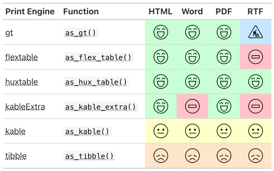
{gtsummary} print engines
Use any print engine to customize table
In Closing
{gtsummary} website
Package Authors/Contributors
Daniel D. Sjoberg
Michael Curry
Emily de le Rua
Joseph Larmarange
Jessica Lavery
Karissa Whiting
Emily C. Zabor
Xing Bai
Esther Drill
Jessica Flynn
Margie Hannum
Stephanie Lobaugh
Shannon Pileggi
Amy Tin
Gustavo Zapata Wainberg
Other Contributors
@ablack3, @ABorakati, @aghaynes, @ahinton-mmc, @aito123, @akarsteve, @akefley, @albertostefanelli, @alexis-catherine, @amygimma, @anaavu, @andrader, @angelgar, @arbet003, @arnmayer, @aspina7, @asshah4, @awcm0n, @barthelmes, @bcjaeger, @BeauMeche, @benediktclaus, @berg-michael, @bhattmaulik, @BioYork, @brachem-christian, @bwiernik, @bx259, @calebasaraba, @CarolineXGao, @ChongTienGoh, @Chris-M-P, @chrisleitzinger, @cjprobst, @clmawhorter, @CodieMonster, @coeus-analytics, @coreysparks, @ctlamb, @davidgohel, @davidkane9, @dax44, @dchiu911, @ddsjoberg, @DeFilippis, @denis-or, @dereksonderegger, @dieuv0, @discoleo, @djbirke, @dmenne, @ElfatihHasabo, @emilyvertosick, @ercbk, @erikvona, @eweisbrod, @feizhadj, @fh-jsnider, @ge-generation, @ghost, @gjones1219, @gorkang, @GuiMarthe, @hass91, @HichemLa, @hughjonesd, @iaingallagher, @ilyamusabirov, @IndrajeetPatil, @IsadoraBM, @j-tamad, @jalavery, @jeanmanguy, @jemus42, @jenifav, @jennybc, @JeremyPasco, @JesseRop, @jflynn264, @jjallaire, @jmbarajas, @jmbarbone, @JoanneF1229, @joelgautschi, @jojosgithub, @JonGretar, @jordan49er, @jthomasmock, @juseer, @jwilliman, @karissawhiting, @kendonB, @kmdono02, @kwakuduahc1, @lamhine, @larmarange, @leejasme, @loukesio, @lspeetluk, @ltin1214, @lucavd, @LuiNov, @maia-sh, @Marsus1972, @matthieu-faron, @mbac, @mdidish, @MelissaAssel, @michaelcurry1123, @mljaniczek, @moleps, @motocci, @msberends, @mvuorre, @myensr, @MyKo101, @oranwutang, @palantre, @Pascal-Schmidt, @pedersebastian, @perlatex, @philsf, @polc1410, @postgres-newbie, @proshano, @raphidoc, @RaviBot, @rich-iannone, @RiversPharmD, @rmgpanw, @roman2023, @ryzhu75, @sachijay, @saifelayan, @sammo3182, @sandhyapc, @sbalci, @sda030, @shannonpileggi, @shengchaohou, @ShixiangWang, @simonpcouch, @slb2240, @slobaugh, @spiralparagon, @StaffanBetner, @Stephonomon, @storopoli, @szimmer, @tamytsujimoto, @TarJae, @themichjam, @THIB20, @tibirkrajc, @tjmeyers, @tldrcharlene, @tormodb, @toshifumikuroda, @UAB-BST-680, @uakimix, @uriahf, @Valja64, @vvm02, @xkcococo, @yonicd, @yoursdearboy, @zabore, @zachariae, @zaddyzad, @zeyunlu, @zhengnow, @zlkrvsm, @zongell-star, and @Zoulf001.
Thank you