Perform Decision Curve Analysis

Diagnostic and prognostic models are typically evaluated with measures of accuracy that do not address clinical consequences. Decision-analytic techniques allow assessment of clinical outcomes but often require collection of additional information may be cumbersome to apply to models that yield a continuous result. Decision curve analysis is a method for evaluating and comparing prediction models that incorporates clinical consequences, requires only the data set on which the models are tested, and can be applied to models that have either continuous or dichotomous results. The dca function performs decision curve analysis for binary outcomes. Review the DCA Vignette for a detailed walk-through of various applications. Also, see www.decisioncurveanalysis.org for more information.

dca(
  formula,
  data,
  thresholds = seq(0, 0.99, by = 0.01),
  label = NULL,
  harm = NULL,
  as_probability = character(),
  time = NULL,
  prevalence = NULL
)

Arguments

formula

a formula with the outcome on the LHS and a sum of markers/covariates to test on the RHS

data

a data frame containing the variables in formula=.

thresholds

vector of threshold probabilities between 0 and 1. Default is seq(0, 0.99, by = 0.01). Thresholds at zero are replaced with 10e-10.

label

named list of variable labels, e.g. list(age = "Age, years")

harm

named list of harms associated with a test. Default is NULL

as_probability

character vector including names of variables that will be converted to a probability. Details below.

time

if outcome is survival, time= specifies the time the assessment is made

prevalence

When NULL, the prevalence is estimated from data=. If the data passed is a case-control set, the population prevalence may be set with this argument.

Value

List including net benefit of each variable

as_probability argument

While the as_probability= argument can be used to convert a marker to the probability scale, use the argument only when the consequences are fully understood. For example, when the outcome is binary, logistic regression is used to convert the marker to a probability. The logistic regression model assumes linearity on the log-odds scale and can induce miscalibration when this assumption is not true. Miscalibration in a model will adversely affect performance on decision curve analysis. Similarly, when the outcome is time-to-event, Cox Proportional Hazards regression is used to convert the marker to a probability. The Cox model also has a linearity assumption and additionally assumes proportional hazards over the follow-up period. When these assumptions are violated, important miscalibration may occur.

Instead of using the as_probability= argument, it is suggested to perform the regression modeling outside of the dca() function utilizing methods, such as non-linear modeling, as appropriate.

See also

net_intervention_avoided(), standardized_net_benefit(), plot.dca(), as_tibble.dca()

Author

Daniel D Sjoberg

Examples

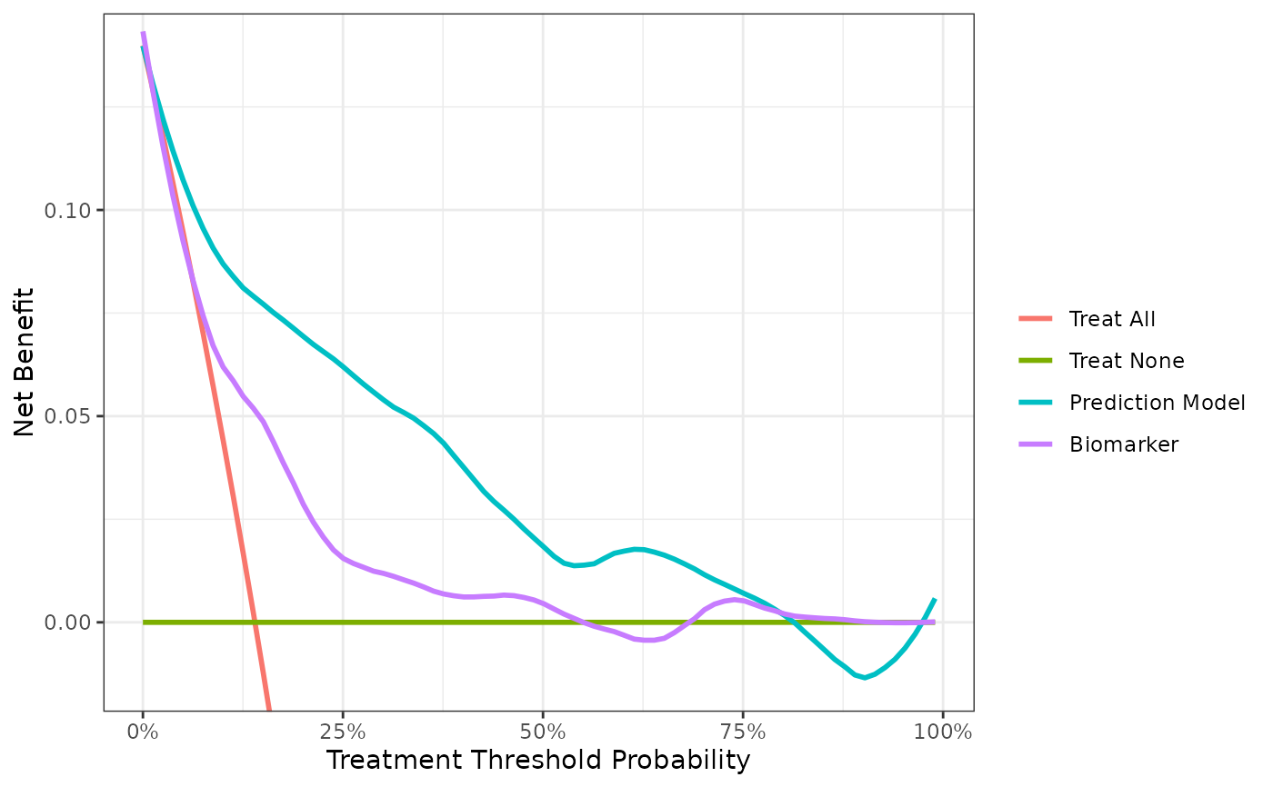
# calculate DCA with binary endpoint
dca(cancer ~ cancerpredmarker + marker,
    data = df_binary,
    as_probability = "marker",
    label = list(cancerpredmarker = "Prediction Model", marker = "Biomarker")) %>%
  # plot DCA curves with ggplot
  plot(smooth = TRUE) +
  # add ggplot formatting
  ggplot2::labs(x = "Treatment Threshold Probability")


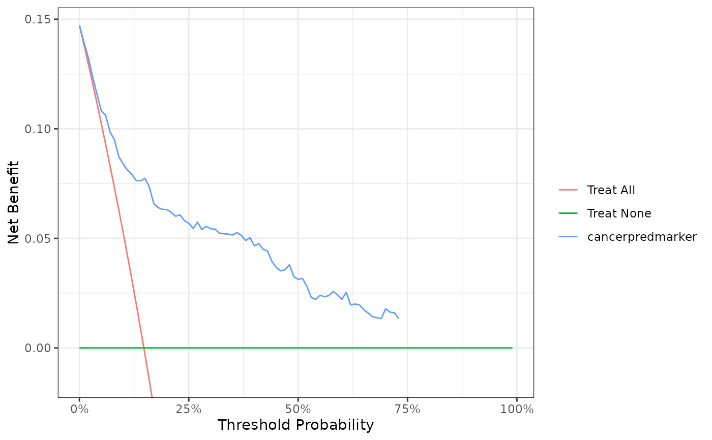
# calculate DCA with time to event endpoint
dca(Surv(ttcancer, cancer) ~ cancerpredmarker, data = df_surv, time = 1)
#> Printing with `plot(x, type = 'net_benefit', smooth = FALSE, show_ggplot_code = FALSE)`