Apply Scales

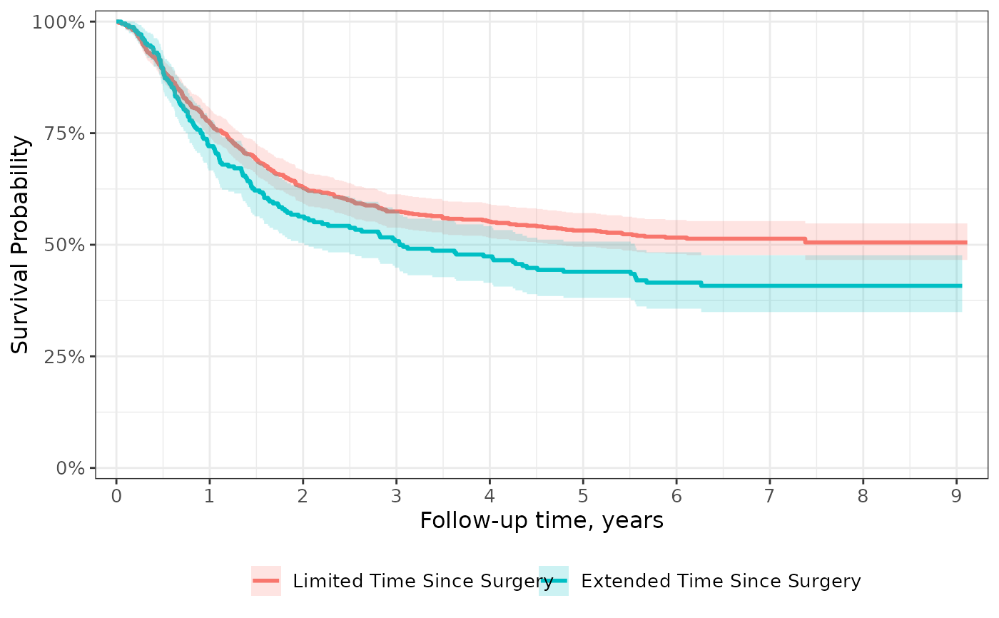
The most common figure created with this package is a survival curve. This scale applies modifications often seen in these figures.

• scale_y_continuous(expand = c(0.025, 0), limits = c(0, 1), label = scales::label_percent()).

• scale_x_continuous(expand = c(0.015, 0), n.breaks = 8)

NOTE: The y-axis limits are only set for survival curves.

If you use this function, you must include all scale specifications that would appear in scale_x_continuous() or scale_y_continuous(). For example, it's common you'll need to specify the x-axis break points. scale_ggsurvfit(x_scales=list(breaks=0:9)).

To reset any of the above settings to their ggplot2 default, set the value to NULL, e.g. y_scales = list(limits = NULL).

Usage

scale_ggsurvfit(x_scales = list(), y_scales = list())

Arguments

x_scales

a named list of arguments that will be passed to ggplot2::scale_x_continuous().

y_scales

a named list of arguments that will be passed to ggplot2::scale_y_continuous().

Value

a ggplot2 figure

Details

Special case: in the risk table, large numbers (with more than 4 digits) may not be shown completely, with some digits truncated outside the plot region. To remedy this, consider adjusting the expand size:

scale_ggsurvfit(x_scales = list(expand = c(0.05, 0)))

This can modify the position of numbers in the risk table and make them all fit in the plot region. The scale of the expand argument differs by cases.

See also

Visit the gallery for examples modifying the default figures

Examples

ggsurvfit <-
  survfit2(Surv(time, status) ~ surg, data = df_colon) %>%
  ggsurvfit(linewidth = 1) +
  add_confidence_interval()

# use the function defaults
ggsurvfit + scale_ggsurvfit()


# specify additional scales
ggsurvfit +
  scale_ggsurvfit(x_scales = list(breaks = seq(0, 8, by = 2)))